Deep Learning for Information Extraction

This is the first part of a series of articles about Deep Learning methods for Natural Language Processing applications. As a use case I would like to walk you through the different aspects of Named Entity Recognition (NER), an important task of Information Extraction. In this first article I will give you an introduction to this topic. I will describe the baseline Deep Learning architecture for Named Entity Recognition, which is a bidirectional Recurrent Neural Network based on LSTM or GRU.

In the coming parts, I will go deeper into the different strategies of extending this architecture in order to improve extraction results. I will also present alternative or complementary strategies. These extensions and alternatives will include many different concepts like pre-trained word embeddings, residual connections, character level embeddings, Conditional Random Field, Temporal Convolutional Neural Networks, ensemble models etc.

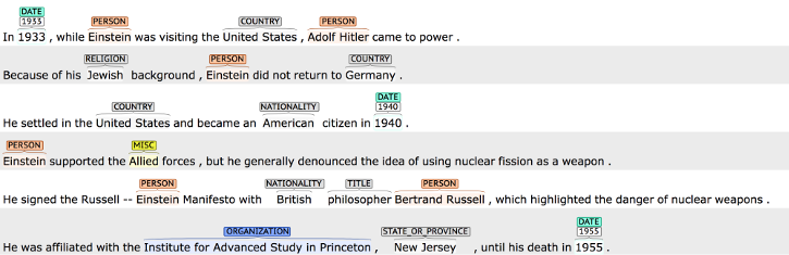
The extraction of relevant information from unstructured documents is a key component in Natural Language Processing (NLP) systems that can be used in many different applications. Named entity recognition (NER) is a specific task of information extraction. It aims the identification of named entities like persons, locations, organizations, dates etc. in text. For example in the illustration below the snippet “Institute for Advanced Study in Princeton” is assigned to the category “ORGANIZATION” and “Bertrand Russell” to the category “PERSON”:

The automatic labelling of a NER system can be used by publishers, libraries or other content providers to tag documents and potentially improve search results. Other obvious applications are recommendation systems and customer support.

NER can also serve as a core component to extract legally relevant information from contracts or other legal documents. The challenge in this case is the identification of deadlines, due dates, terms, conditions, contract parties etc. Similarly, the extraction of accounting information from invoices or tax assessments requires the recognition of amounts, tax rates, due dates, bank information etc.

Until recently automatic extraction systems, especially for use cases like the latter two examples, were not able to provide reliable results, consistently. This is mainly due to the complexity of these kind of documents and the low error tolerance demanded by law. Tasks like the ones described require a relative high level of language and domain specific context understanding. Hence, many companies often still deploy humans for these kind of tasks.

The first approaches to tackle the NER task were based on manually crafted sets of rules. Purely rule-based methods often work well only within a very narrow specific domain. Rules needs to be updated and adjusted regularly. The decision tree is usually growing and getting more and more complex with time. Hence, updates and maintenance of these systems become more and more laborious, time consuming and error prone.

Potential solution to this generalization problem is the use of statistical models based on Machine Learning (ML). One of the most successful ML methods before the resurrection of neural networks were models based on Conditional Random Fields (CRF). The performance of these models heavily depended on hand-crafted features which requires a lot of domain specific knowledge and often a deep understanding of linguistics.

In the recent years the development in this area has been dominated by Deep Learning (DL) methods. DL models are usually trained end-to-end, i. e. extensive manual feature engineering is not required any more. The lower layers of the Deep Neural Network learn the optimal feature representation by itself, while the higher layers act as the final classifier. The challenge nowadays is merely the choice or the construction of the right network architecture, the definition of an appropriate cost function and the gathering of a lot of data.

Recurrent Neural Networks (RNN) have been the preferred choice of DL architectures for the NER task amongst researchers and practitioners. In particular, RNNs based on Long Short Term Memory (LSTM) cells or Gated Recurrent Unit (GRU) cells. Recently, also models based on one-dimensional Convolutional Neural Networks (CNN), the so called Temporal CNN (TCN) are reported to give competitive results. Currently, the most successful architectures often consist of a multi-layer RNN or TCN with a CRF as the final layer.

Data Acquisition

Procurement of sufficiently large amount of (annotated) data is still the greatest obstacle to the successful application of DL. The number of documents needed depends on many parameters, mainly on the complexity of the problem and the quality of the annotations. It can start from a few hundred and can go up to a more than hundred of thousands. One successful strategy might be to start with a couple of thousand samples and keep on collecting more data over time until one can identify saturation of the performance metric.

Preprocessing

Paper documents need to be scanned first before the character sequence can be extracted using an Optical Character Recognition (OCR) System. Digital documents in PDF, JPG, PNG or any other image format are sent directly to the OCR system. Character sequences in PDF documents with embedded text or other text formats can be read out directly.

In the next step NLP tools like NLTK or spaCy can be used to transform the character sequences to sequences of normalized tokens. Tokens are the smallest semantic unit of a sentence, usually words.

Annotations

The extraction techniques discussed in this article belong to the class of so called supervised learning methods. In contrast to unsupervised learning methods this kind of method requires annotated data sets, i. e. data sets that already include the truth information of the labels. Usually, the tags need to be annotated by humans.

The specific labels depend on the respective application. As an example we can choose the ones matching our example in the image above:

• COUNTRY
• DATE
• PERSON
• ORGANIZATION
• NATIONALITY
• TITLE
• STATE_OR_PROVINCE
• MISC
• RELIGION
• O (none of the other labels)

Exactly one label is assigned to each token of the sequence. The BILOU scheme extends the basic scheme by adding prefixes:

• B - Begin: first token of entity
• I - Inside: token inside entity
• L - Last: last token of entity
• U - Unit: single token of entity
• O - Outside: outside of any named entity

Given the input sequence:

the label sequence in the BILOU scheme looks like this:

Using the most simple IO scheme the label sequence would look like this:

The BILOU scheme is much more expressive than a simple IO scheme and often leads to better extraction results. But on the other hand it takes much more effort and time to annotate the data.

Recurrent Neural Network

Currently, RNNs are the most popular Deep Learning model to solve the NER task. A simple RNN cell looks like this on the left:

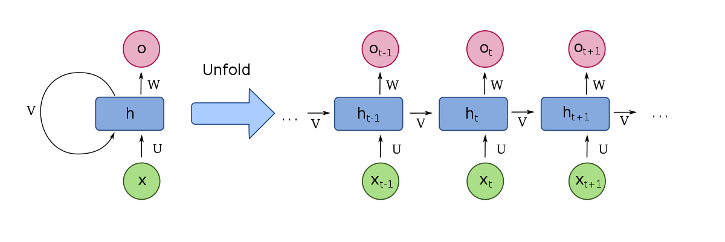
x_i: inputs
h_i: hidden states (memory)
o_i: outputs
U: input weights
V: hidden weights (recurrent connection)
W: output weights

The input is processed sequentially as you might better see on the unfolded representation on the right. Characteristic for RNNs is that all weights/parameters are reused for each iteration step. Only the hidden state is updated dependent on the previous hidden state and the current input. The hidden state works as the memory of the network, that stores the most important information from the previous inputs.

LSTM & GRU Cells

Unfortunately, simple RNNs have a very short memory, due to the issue of vanishing gradients. More complicated cell architectures try to solve the short memory problem. The most famous one is probably the Long Short Term Memory (LSTM) cell:

It uses a gated cell architecture to update and forget information selectively in the network memory (cell and hidden states). The Gated Recurrent Units (GRU) have a slightly simpler architecture (and only one hidden state):

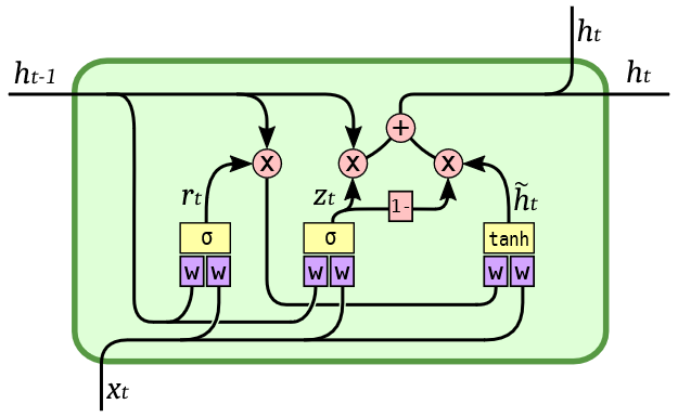
GRUs are usually faster than LSTMs, while still often have competitive performances for many applications.

Bidirectional RNN

A simple example for a Deep Learning NER system is a one layered bidirectional RNN based on LSTM or GRU cells, in this case GRUs:

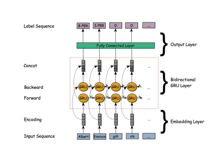
A bidirectional RNN consists of a so called forward layer and a backward layer. The input sequence is fed to the forward layer in the regular way, while in the backward layer the input is processed in the reverse order, starting from the last word, then proceed to the next to last word and so on up to to first word.

The hidden states are then concatenated for each token generating an intermediate representation sequence. Hence, for each intermediate representation the information from the sequence before and after the respective token are taken into account. That means for each iteration step the network has access to the complete document and can deduce the right label from that information.

This is an example for the implementation of a bidirectional GRU network in PyTorch:

import torch.nn as nn

class RNN(nn.Module):
    def __init__(self, embedding_dim, hidden_dim, vocab_size, tagset_size, batch_size=1, 
                 num_layers=1, bidirectional=True):
        super(RNN, self).__init__()
        
        self.num_layers = num_layers
        self.hidden_dim = hidden_dim
        self.num_directions = 2 if bidirectional else 1
        
        self.word_embeddings = nn.Embedding(vocab_size, embedding_dim)        
        self.gru = nn.GRU(embedding_dim, hidden_dim, num_layers=num_layers,
                          bidirectional=bidirectional)
        self.hidden = self.init_hidden(batch_size)
        self.hidden2tag = nn.Linear(hidden_dim * self.num_directions, tagset_size)        
        
    def init_hidden(self, batch_size=1):
        return (torch.zeros(self.num_layers * self.num_directions, 
                            batch_size, self.hidden_dim))
    
    def forward(self, sentence):
        embeds = self.word_embeddings(sentence)
        gru_out, self.hidden = self.gru(embeds, self.hidden)
        tag_scores = self.hidden2tag(gru_out)
        
        return tag_scores

In PyTorch a custom network class is inherited from the abstract class nn.Module, where the methods __init__() and forward() have to be defined. In __init__() you should initialize and instantiate all necessary elements of your network. The order does not matter, but as good style you should generate them in same order as they will run in the forward() method.

In our case we will create four elements:

1. word_embeddings: The embedding layer is used for encoding sequences of tokens. It maps a word index to an n-dimensional word vector. Note that the weights of this lookup table can be learned during the training. nn.Embedding(vocab_size, embedding_dim) generates such a lookup table, where vocab_size denotes the size of the size of the vocabular and embedding_dim the dimension of the output vector.
2. gru: Generates one or multiple layers of GRU cells. embed_dim indicates the input dimension, while hidden_dim is the output dimension. The number of layers can be set optionally with num_layer. With the argument bidirectional you can choose whether to implement each layer as bidirectional layer or not. The module GRU() expects input dimensions with the shape (sequence length, batch size, input dimension) and returns a sequence of all hidden states plus the last hidden state.
3. hidden: The last hidden state needs to be stored separately and should be initialized via init_hidden(). Batch sizes can be set dynamically.
4. hidden2tag: A feed forward layer, which takes as input an tensor with dimensions (sequence length, batch size, hidden dimension * 2). The factor 2 takes into account bidirectional layers. The output tensor has the dimensions (sequence length, batch size, number of labels).

The forward() method defines the actual forward processing sequence. An example for creating an instance of the just defined bidirectional GRU network, the initialization of the hidden state and a call of one forward pass is given here:

model = RNN(300, 200, 50000, 8, batch_size=1, num_layers=1, bidirectional=True)
model.hidden = model.init_hidden(1)
tags = model(input_seq)

Autograd, Backpropagation and Training

PyTorch uses the package autograd to generate a directed acyclic graph (DAG) dynamically. That means for each forward pass a graph is generated depending on the actual sequence. This is in contrast to static graphs (as in frameworks like Tensorflow), where the graph is generated only once at the beginning and cannot be modified anymore. Dynamic graphs have advantages if you want to run more complex and flexible networks, also the debugging is much more straight forward. This makes them particularly popular amongst researchers and NLP engineers. Static graphs have their upside when it comes to optimization and deployment.

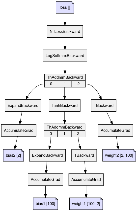
PyTorch tensors store the history of the way they were generated (tensors and operators). autograd uses this information to do automatic differentiation. During the forward pass it generates a graph with the tensors as nodes and the operators as edges, which can be used for backpropagation:

An example for a training loop is given here:

import torch.optim as optim

loss_function = nn.CrossEntropyLoss()
optimizer = optim.SGD(model.parameters(), lr=0.1) 

for epoch in range(100): 
    model.zero_grad()
    
    model.hidden = model.init_hidden(10)
    tags = model(x_input)
    
    loss = loss_function(tags.view(-1, tagset_size), y_true.view(-1))
    loss.backward()
    optimizer.step()

For our multilabel classification problem we choose CrossEntropyLoss() as the loss function. PyTorch provides different optimizer algorithms in the module torch.optim, one of them is stochastic gradient descent (SGD). The parameters of the network to be optimized is passed to SGD(). An optional parameter is the learning rate (lr). In the training loop we start with resetting all gradients of the graph (zero_grad()). Then we initialize the hidden state and run one forward pass. The loss value is obtained by comparing the network output and the truth information. The gradients are calculated by calling backward() and all weights are updated via backpropagation (optimizer.step()).

Outlook

In the next part of the series I will discuss the evaluation of our models and how we can use pre-trained word embeddings to improve the results of the extraction.