
The simulation of behavior models, for instance using YAKINDU Statechart Tools, is an important feature for evolutionary, model-based software development. Imagine that you can see the simulation of the behavior model side-by-side with the behavior of the system at the same time. How would it be if you could interactively change the behavior model, properties of the system or the environment of the system during simulations to explore different solutions?
In the following video, you see what I have prototypically built to get a feeling for such an interactive 3D visualization and simulation environment. I used YAKINDU Statechart Tools (SCT) for simulating the system behavior using state machines, which you see on the right side of the video.

For physics simulation and visualization of the system in its environment, I used the Unity game engine, which you see on the left side. The data of both tools is synchronized to achieve a co-simulation of the tools.
Why Interactive 3D Visualization and Simulation?
Before we are going to have a closer look at my proof of concept for an interactive 3D visualization and simulation using YAKINDU Statechart Tools and the Unity game engine, we are first discussing potential benefits of simulation, visualization, and interactivity.
What are potential benefits of simulation?
Simulations allow developers to test their solutions early, for instance, by overcoming missing components and missing prototypes. There are specialized simulation tools for a variety of requirements ranging from tools for physical simulations to tools for simulating the output of pins of a chip. In addition to the system itself, the system's environment can also be simulated - including rarely occurring and unusual situations. For an early feedback, simulation must not be perfectly accurate. It is enough if the approximations, which are used for the simulations, are sufficiently accurate with respect to the functional and non-functional requirements of the system. Early and frequent feedback about the validity and quality of a solution is essential to continuously develop in the right direction. By thus avoiding big changes in later phases of system development, simulations can help to reduce system development costs and time-to-market.
What are potential benefits of visualization?
Data visualizations of system behavior over time generally give a quick and easy to grasp overview of the quality of solutions. After all, a picture is worth a thousand words. 2D/3D Visualizations of system behavior within its environment make solution exploration even more tangible for developers. Moreover, non-technical stakeholders can much better assess if the system behavior meets their requirements, when they can actually see the system behavior compared to when they receive indirect feedback based on abstract tests or data. Different scenarios can be visualized to clarify questions and evaluate possible solutions together with developers. Consequently, non-technical stakeholders are more likely to contribute good feedback for further development. One big advantage of system behavior visualization is thus the reduction of possible misinterpretations and misunderstandings, which are caused by assumptions to cognitively map indirect feedback, such as abstract data, into system behavior. When visualization is used together with simulations, flaws, which otherwise might only be determined when tests with real prototypes are conducted, might be found considerable earlier. As a result, visualization can also help to reduce system development costs and time-to-market.
What are potential benefits of interactivity?
Interactive changes of behavior models, simulation parameters and system environments during simulations facilitate an explorative solution development process and solution tuning. Developers do not have to wait for changes to take effect, for instance due to the compilation process and restart of simulations. Instead, developers instantly see how the system behavior changes based on their modifications. An iterative, model-driven development process can thus be potentially performed more efficiently using interactive changes.
Car Distance Keeper System
For the proof of concept of an interactive 3D visualization and simulation, we are building a car distance keeper system. As depicted in the image above, there are two cars that will be driving along a racetrack. The back car is following the front car in a defined distance. To provide a pleasant driving experience for the car occupants, the distance keeper system must smoothly accelerate and decelerate. We can expect a trade-off between acceleration change smoothness and tolerance concerning the distance to the front car, which we need to consider for collision avoidance.
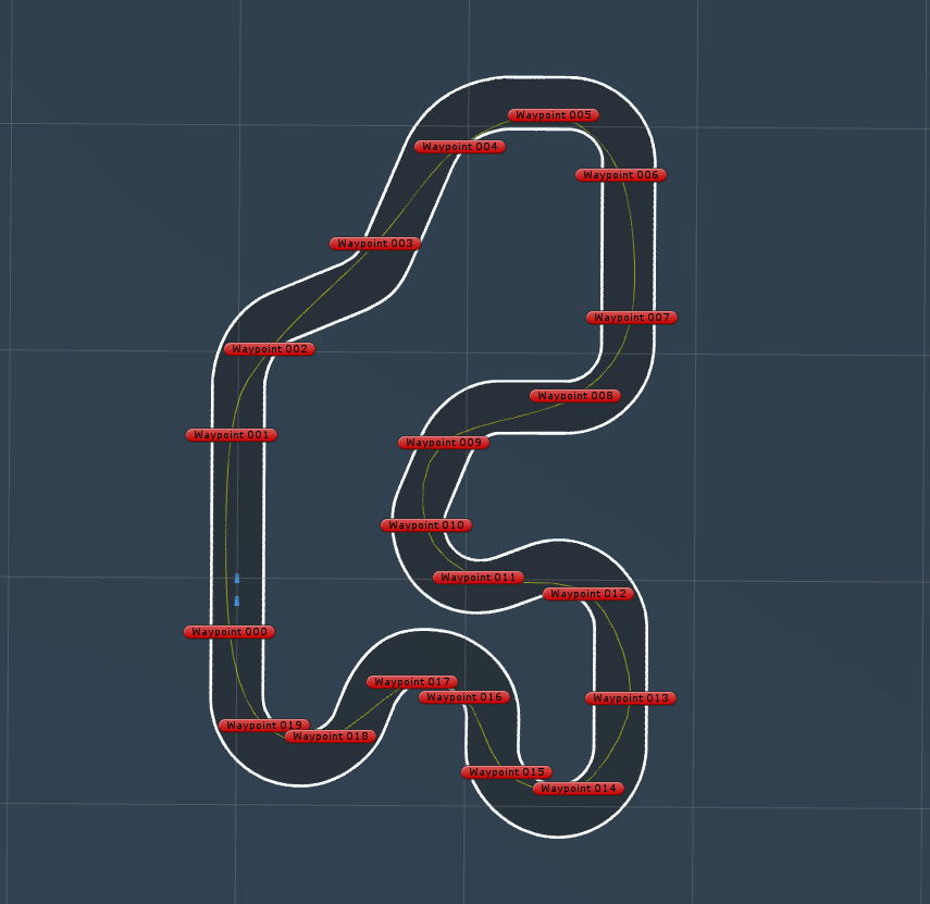
Instead of controlling the front car using keyboard input, we use a script to drive the car. The script will automatically control steering and acceleration/deceleration. The front car thus follows a track, which is defined by several waypoints (see image below).
Behavior Modelling and Simulation
We are using the YAKINDU Statechart Tools to model and simulate the behavior of the car distance keeper system. You can find more information on how to use state machines for your modelling and how to simulate a statechart model with YAKINDU Statechart Tools in our blog. The following listing shows the Car interface, which defines all required values for our model:
@CycleBased(15)
interface Car:
    // Desired distance to front car
    var readonly targetDistance: real = 10.0
    // Current distance to front car
    var distance : real = targetDistance
    // Current acceleration or deceleration
    // (-1 maximum deceleration to +1 maximum acceleration)
    var acceleration : real = 0.0
    // Smoothing factor for acceleration
    var readonly accelerationSensitivity : real = 0.25
    // Smoothing factor for deceleration
    var readonly brakeSensitivity : real = 0.5

    // Angle between back car heading and direct connection
    // line between the back and front car
    var targetAngle : real = 0.0
    // Current steering angle
    // (-1 maximum steering to the left to
    //  +1 maximum steering to the right)
    var steering : real = 0.0
    // Smoothing factor for steering
    var readonly steerSensitivity : real = 0.05
Please note that readonly means that the variables must not be changed in the state machine, but it is possible to change the values during simulation. Therefore, readonly acts as a safeguard without restricting our possibilities for interactive changes during simulation.
Acceleration Behavior Model
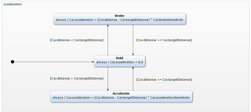
Now that the Car interface is defined, let's model the acceleration behavior. We want a simple model consisting of three states:
- Brake: Whenever the current
distanceto the front car is smaller than thetargetDistance, the system needs to brake the car. - Hold: Whenever the current
distanceto the front car equals thetargetDistance, the system needs to hold the current velocity of the car. - Accelerate: Whenever the current
distanceto the front car is greater than thetargetDistance, the system needs to accelerate the car.
The acceleration magnitude is based on the deviation of the current distance from the targetDistance, which is multiplied with the corresponding smoothing factors brakeSensitivity and accelerationSensitivity. This model is of course far too simplistic for a real system, such as an Adaptive Cruise Control (ACC), but it is sufficient for illustration purposes in the context of this blog post. Here is an image of the final acceleration behavior model:
Steering Behavior Model
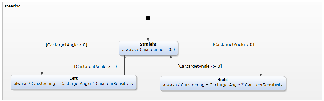
Next, we need to model the car steering behavior. One simple way to achieve that the back car is following the front car is to align the tires of the back car with the direction towards the front car (i.e. according to the targetAngle). As the movement range of car tires is limited and we want to avoid a shaky driving experience, we use the steerSensitivity smoothing factor. Analogous to the acceleration model, we are using three states for the steering behavior model:
- Left: Whenever the front car is to the left (i.e.
targetAngle< 0), the system needs to steer the car to the left. - Straight: Whenever the front car is directly in front (i.e.
targetAngle= 0), the system needs to keep the car straight. - Right: Whenever the front car is to the right (i.e.
targetAngle> 0), the system needs to steer the car to the right.
Yes, again this model is too simplistic for a real system and you could achieve the same behavior with one state instead of three. However, for visualization purposes it is better to have three logical states so that the active model state indicates the steering direction. An illustration of the final steering behavior model is shown in the following image:
Although we can now simulate both behavior models using YAKINDU Statechart Tools, we would need to manually enter values for the current distance to the front car as well as the targetAngle towards the front car. That would not be a very dynamic simulation experience. To create a dynamic simulation, we need to simulate the driving physics and to visualize the car while it is driving.
Physics Simulation and Visualization
The Unity game engine with its standard assets example project contains everything that we need. It includes a 3D scene consisting of a car on a racetrack. The car is controlled by a script to follow the racetrack based on waypoints, as shown in the "Car Distance Keeper System" section above. Moreover, there is a CarController script, which provides simple driving physics together with the physics engine that is used by Unity. We just need to add a second car from the standard assets.
Now we have, on the one hand, a simulation of the driving physics together with a 3D visualization of the car within its environment. On the other hand, we have the simulation of our acceleration and steering behavior for the back car. The only problem is that both simulations are performed by different tools and thus totally isolated from each other. Consequently, the next key challenge is to let both simulation tools work together.
Co-Simulation
For the co-simulation using both tools, we need to constantly exchange the simulation data. One possibility is to use the YAKINDU Communication Protocol (YaCoP), which can be made available through a plugin for the YAKINDU Statechart Tools. Currently, the YaCoP plugin is not included in the YAKINDU Statechart Tools. If you want to get YaCoP to built this proof of concept or for experimentation, please contact us. YaCoP sends simple messages over a TCP/IP socket connection. The YaCoP message format consists of three comma-separated values: (1) a # placeholder, (2) the variable name, and (3) the variable value. For instance, when the Car.acceleration value was changed to 0.12345 in the acceleration behavior model simulation, the following message is send over the socket connection:
#,Car.acceleration,0.12345
If this message would be received instead, the YaCoP plugin would set the value of the Car.acceleration variable of the acceleration behavior model simulation to 0.12345.
Data Binding in Unity
All that is left is to implement the data binding on the Unity side. The CarAIController script acts as our basis for a data binding script in C# and is adapted as follows:
using System;
using System.Net.Sockets;
using UnityEngine;

namespace UnityStandardAssets.Vehicles.Car
{
    [RequireComponent(typeof (CarController))]
    public class CarSimulationControl : MonoBehaviour
    {
        [SerializeField] private Transform m_FrontCar;

        [SerializeField] private float m_SteerSensitivity = 0.05f;

        [SerializeField] private string m_YacopIp = "127.0.0.1";
        [SerializeField] private int m_YacopPort = 12345;

        private CarController m_Car;

        private TcpClient m_YacopClient;
        private NetworkStream m_YacopStream;

        private float m_Acceleration = 0.0f;
        private float m_Steering = 0.0f;

        private void Awake()
        {
            m_Car = GetComponent();
        }

        // Establish TCP/IP socket connection to the YaCoP plugin on start
        private void Start()
        {
            m_YacopClient = new TcpClient(m_YacopIp, m_YacopPort);
            m_YacopStream = m_YacopClient.GetStream();
        }

        // Close TCP/IP socket connection to the YaCoP plugin on destroy
        private void OnDestroy()
        {
            m_YacopStream.Close();
            m_YacopClient.Close();
        }

        // Process all incoming YaCoP messages to update acceleration and steering
        private void ProcessYacopStreamData()
        {
            while (m_YacopStream.DataAvailable)
            {
                byte[] buffer = new byte[1024];
                int bytes = m_YacopStream.Read(buffer, 0, buffer.Length);
                string data = System.Text.Encoding.UTF8.GetString(buffer, 0, bytes);
                foreach (string message in data.Split('\n'))
                {
                    string[] fields = message.Split(',');

                    if (fields.Length < 3)
                        continue;

                    string name = fields[1];
                    string value = fields[2];

                    if (name == "Car.acceleration")
                    {
                        m_Acceleration = ParseFloat(value);
                    }
                    else if (name == "Car.steering")
                    {
                        m_Steering = ParseFloat(value);
                    }
                }
            }
        }

        private float ParseFloat(string value)
        {
            try
            {
                return float.Parse(value);
            } catch (FormatException e)
            {
                return 0;
            }
        }

        // Send YaCoP message to update given value in behavior model simulation
        private void UpdateSimulationValue(string name, string value)
        {
            byte[] yacopMessage = System.Text.Encoding.UTF8.GetBytes("#," + name + "," + value + "\n");
            m_YacopStream.Write(yacopMessage, 0, yacopMessage.Length);
        }

        private void UpdateSimulationValue(string name, float value)
        {
            UpdateSimulationValue(name, value.ToString());
        }

        private void FixedUpdate()
        {
            // Read data from behavior model simulation
            ProcessYacopStreamData();

            // Clamp steering and adjust sign based on forward/backward movement
            float steer = Mathf.Clamp(m_Steering, -1, 1) * Mathf.Sign(m_Car.CurrentSpeed);
            // Clamp acceleration
            float accel = Mathf.Clamp(m_Acceleration, -1, 1);

            // Use car controller to move the car based on steering and acceleration
            m_Car.Move(steer, accel, accel, 0f);

            // Calculate distance to front car
            Vector3 offset = m_FrontCar.position - transform.position;
            float distance = offset.magnitude;
            // Calculate local angle towards front car
            Vector3 localTarget = transform.InverseTransformPoint(m_FrontCar.position);
            float targetAngle = Mathf.Atan2(localTarget.x, localTarget.z) * Mathf.Rad2Deg;

            // Update behavior model simulation data
            UpdateSimulationValue("Car.distance", distance);
            UpdateSimulationValue("Car.targetAngle", targetAngle);
            UpdateSimulationValue("Car.steerSensitivity", m_SteerSensitivity);
        }
    }
}
The FixedUpdate callback handles the three main tasks of the controller. First, all incoming YaCoP messages are processed to update the m_Acceleration and m_Steering variables of the Unity script with respect to the running behavior model simulation. Second, the car controller component is used to move the car based on the updated steering and acceleration parameters. Third, the distance towards the front car as well as the targetAngle towards the front car are determined based on the previous physics update and then sent together with the m_SteerSensitivity over the YaCoP socket stream to update the behavior model simulation state.
Starting the Co-Simulation
Finally, we need to ensure the right configuration for the YAKINU Statechart Tool simulation. In the run configurations, make sure that the YAKINDU YaCoP Launcher is used and the YaCoP port is set to 12345 (which is the default setting).
Let's see the interactive 3D visualization and co-simulation of the car distance keeper system in action. How does it compare to what you have imagined at the beginning of the blog post?
Interactive Changes
Both Unity and YAKINDU Statechart Tools support interactive parameter changes during simulations. So once the co-simulation is in place, interactive changes can be applied to all bound simulation parameters without any extra effort. Let's start by playing around with the steering sensitivity on the Unity side:
Now, let's play with the distance to the front car on the YAKINDU Statechart Tools side:
Interactively changing the model parameters helps to get a sense for suitable parameter ranges. At a certain time, however, you will need to ensure that the model parameters fulfil all relevant system requirements.
Model Parameter Tuning
In this section, we want to tune the accelerationSensitivity parameter to fulfil the following two requirements for the car distance keeper system:
- Back car needs to follow front car in a defined distance ± 5m
- Driving experience must be pleasant for car occupants (i.e. low acceleration variation and avoiding switches between full throttle and braking)
The defined distance between the cars is 10m and we set the brakeSensitivity to 0.5. If conditions must be checked over a longer period of time, it can be helpful to look at overview graphs that aggregate the data. Therefore, both distance and acceleration is recorded during two rounds around the racetrack. We are only interested in the situation where the cars are driving, so we remove the first round with the start from a standing position. This procedure is repeated for the following accelerationSensitivity values: 0.05, 0.1, 0.15, 0.2, 0.25, 0.3. By interactively playing with sensitivity, it became clear that the car is already abruptly switching between full throttle and braking at a value of 0.3, so we do not have to check higher values.
Here are the plots for the distance to the front car over time:
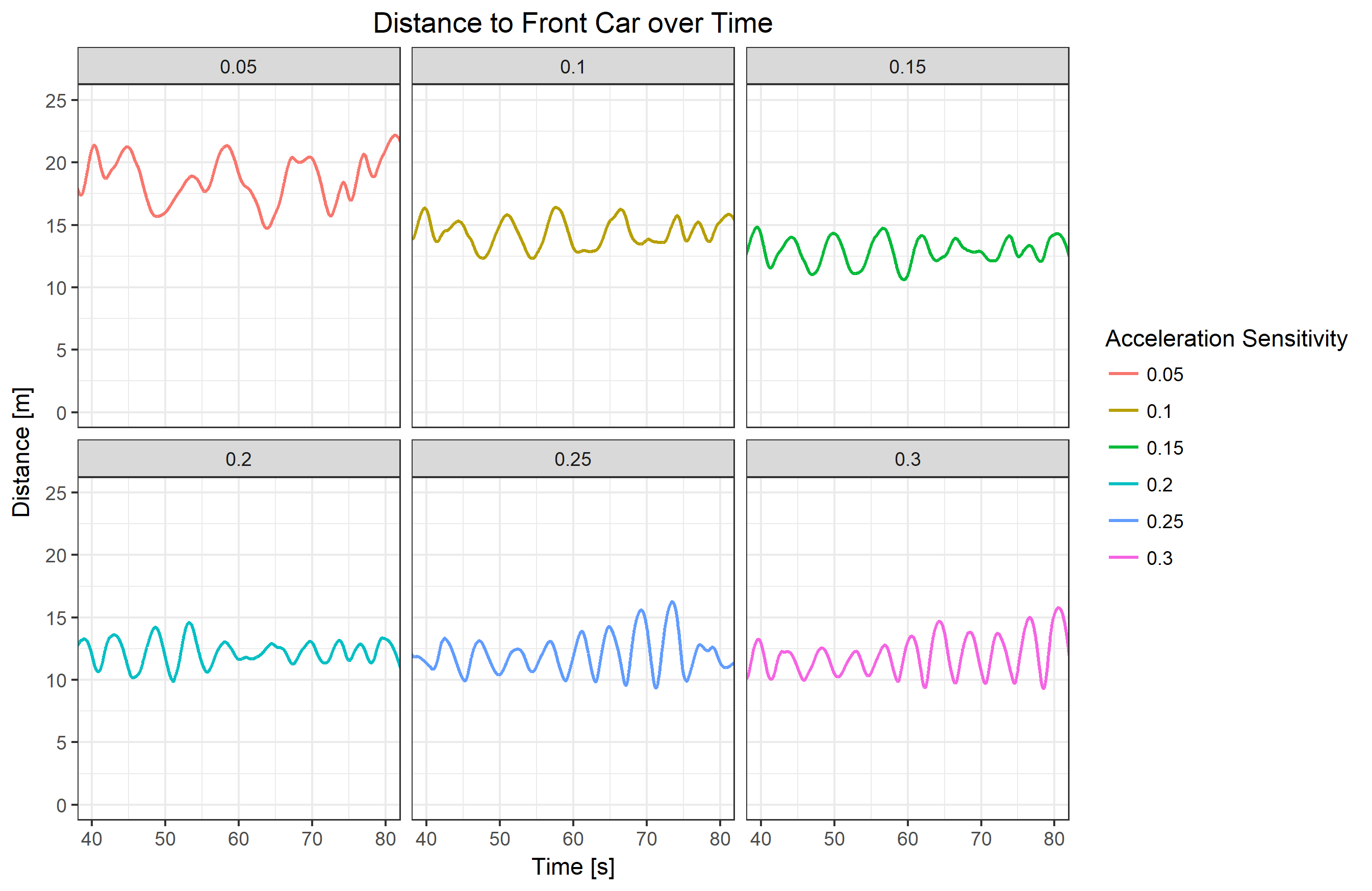
Up until a sensitivity of 0.2, the actual distance to the front car gets smaller. For higher sensitivities, there are some ripples around the 60-80 seconds' area, which again increases the distance. Let's aggregate the data in a boxplot to have a better overview, which sensitivity values fulfil the distance requirement:
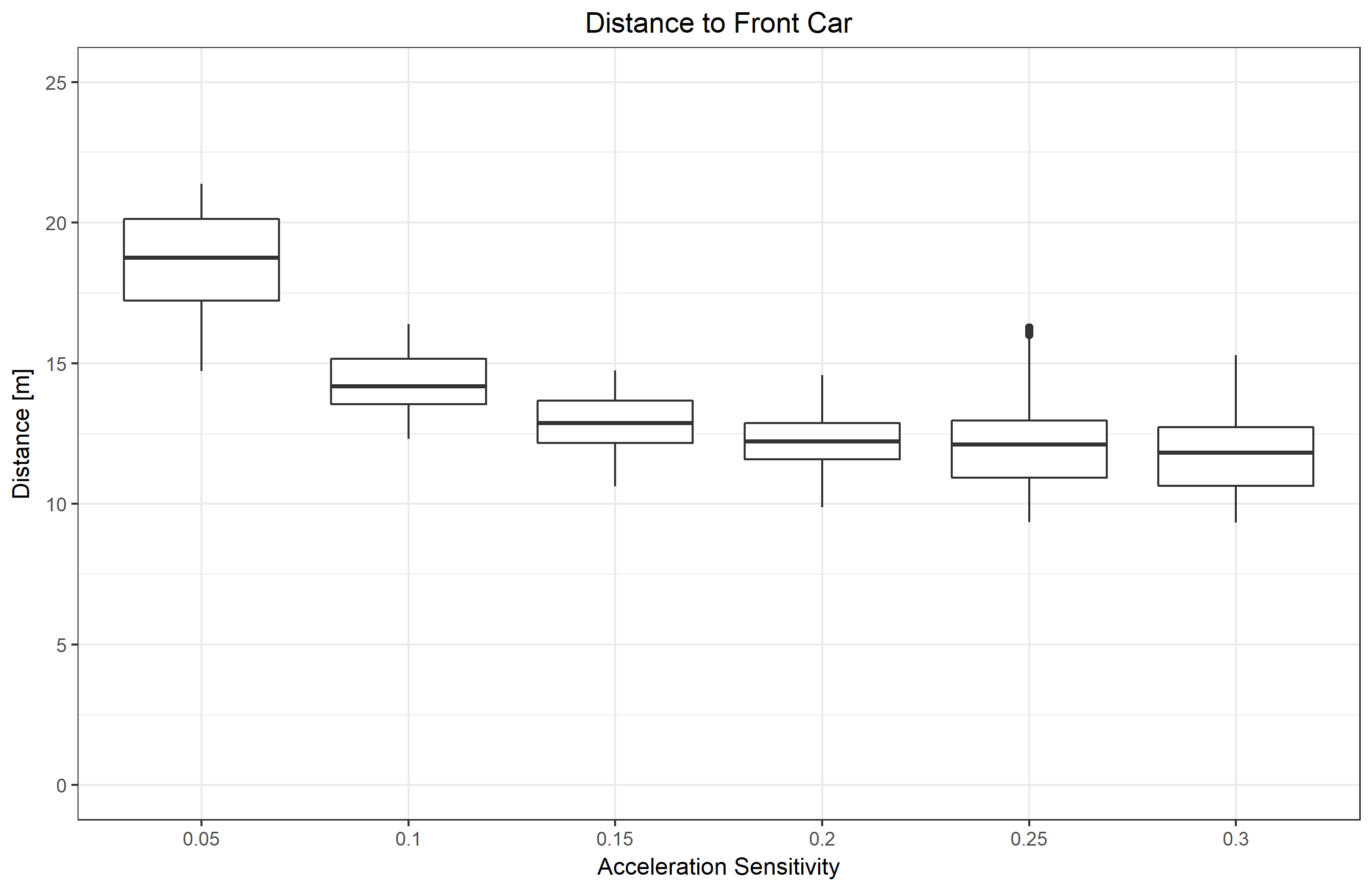
From the boxplot, it is clear that the sensitivities 0.15 and 0.2 are fulfilling the distance requirement 10±5m. For a sensitivity of 0.2, the actual distance to the front car is closer to the defined distance and the distance variation is lower. To decide between the two, we have a look at the acceleration values over time:
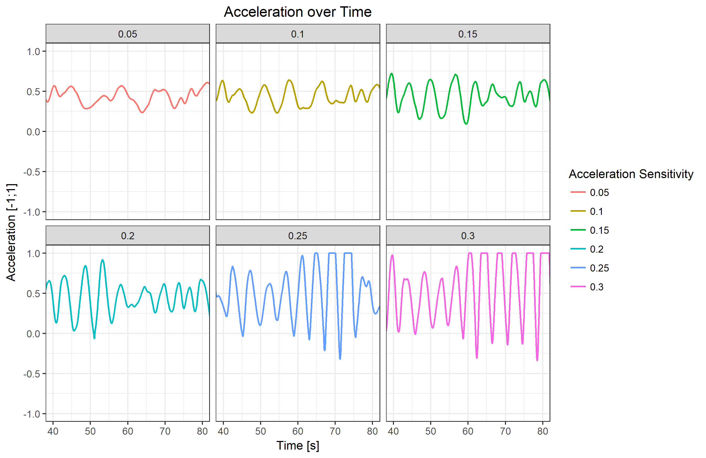
In the case of a sensitivity of 0.2, there seems to be stronger acceleration changes. Still, the car is never driving with full throttle. Let's again aggregate the data in a boxplot to have a better overview:
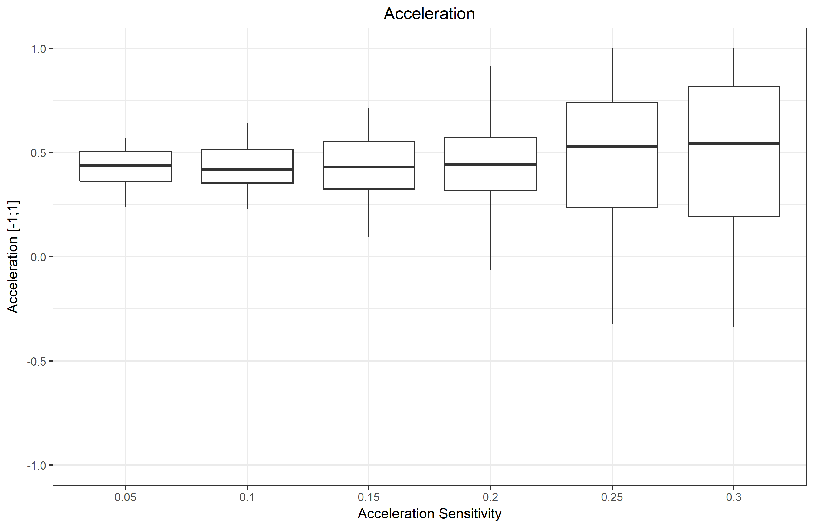
For a sensitivity of 0.15, the brake is actually never used to control the car, whereas it is used in the 0.2 case. Moreover, the acceleration variation as well as the range between minimum and maximum is higher for the sensitivity of 0.2 case. What is better probably depends on the individual taste of a person. I'll leave it up to you to decide if you prefer a more comfortable or a sportier driving experience or even investigate some further intermediary sensitivities.
Conclusions
In this blog post I started with discussing some potential benefits of using simulations, visualizations and interactivity during system development. I showed how to create an interactive 3D visualization and simulation for a car distance keeper system using YAKINDU Statechart Tools and the Unity game engine. The ability to interactively change parameters and receiving a direct feedback facilitates an explorative and iterative development process. Finally, I outlined one possible way to use simulation data for model parameter tuning.
What if you want to use another simulation tool instead of Unity? As long as you can extend the simulation tool with a TCP/IP socket communication to exchange simulation data via YaCoP, you can combine any simulation tool with YAKINDU Statechart Tools. It is also not necessary to visualize the system, so just leave it out if you do not need it.
What's next? We are currently working on co-simulation features. Our plans are, among others, to investigate how co-simulation can be performed with a variety of simulation tools. For instance, standards such as the Functional Mock-Up Interface (FMI) provide tool independent means for co-simulation. In this context, it is also important that the data binding and life cycle management for the co-simulation is automatically generated by the simulation tools to avoid manual wiring as done for Unity in this blog post. Another interesting topic is to support varying simulation speeds to allow developers to quickly perform a large amount of simulation runs, for instance in a headless mode. Therefore, it is essential that simulation runs are recorded and can be replayed later to further analyze certain runs.
Remember how you have imagined an interactive 3D visualization and simulation environment and then compare it with what I have built and what we have planned. Are we missing something? Do you have further ideas? Do you want to rebuild the presented example yourself? Any kind of feedback is welcome, contact us and let us know what you are thinking!

Comments